Getting Started with the NanoVNA -part 1

This post now includes some edits based on user feedback[in green italic]

What is a VNA?

The Vector Network Analyser is an essential piece of test equipment that no RF engineer should be without. If you have previously worked with Electronics at low frequencies, you may consider a good DMM or Oscilloscope your best friend. RF Engineers would gladly trade both a scope for a good VNA!

A good VNA is an expensive bit of kit. Many years ago, a good one would probably cost you as much as a fairly nice house. Nowadays, you can pickup something really good for the price of a nice car. Note, High-end VNAs can still sell for between $100K and $1M. I will use the term ‘professional VNA’.

“What’s it’s dynamic range again?”

Luckily, there are cheap alternatives now, such as the NanoVNA. It doesn’t hold a candle to the performance of a instrument grade piece of kit, but for the price, and used with care, it’s not too bad.

So, what does it do…

A VNA is designed to inject a known frequency and amplitude source signal into a RF port and measure the relative amplitude and phase of this signal when received at a number at one, or more of it’s ports.

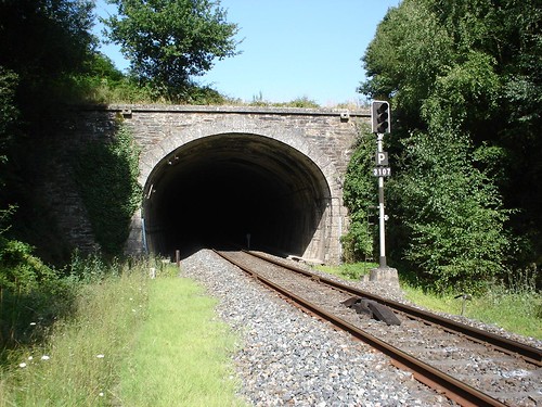
“Atrévete a Entrar…”by Hadrian Fernandez is licensed under CC BY-NC-SA 2.0

That sounds pretty complex, but it’s really not. An analogy might help. For an alternate analogy take a look at KirbyMicrowaves site. Say you are standing at on end of a dark train tunnel and want to know something about what is inside. We will assume that you don’t want to go in, because, well, your scared of the dark and don’t want to be hit by a train.

You have a great idea! What happens if I shout into the tunnel and have a friend listen at the other end. We might be able to work out the length from the volume and delay(you were careful to synchronise watches) of the received sound. Perhaps, we can detect a difference between the high and low pitch sounds. Maybe there is some material in there that is absorbing the high pitch noises, or closed service tunnel that has created a resonance. You have just measured the ‘thru’ characteristics of this tunnel. In VNA parlance, we will call this a S21 measurement, meaning we have made a measurement of a signal at port 2(your friend) of a signal injected at port 1(your beautiful voice).

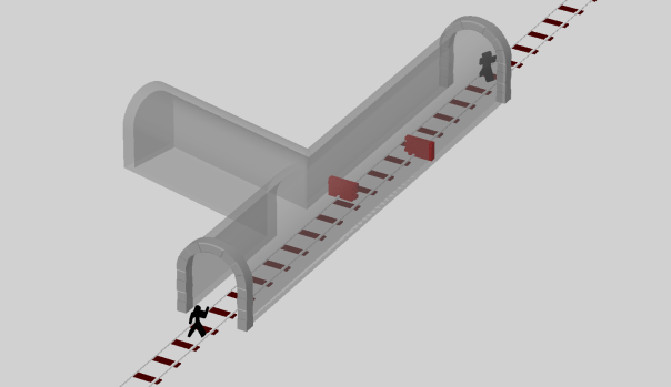
“Dude, Some moron built a wall inside this tunnel!!”; “Yeah, I think the author was trying to illustrate a point about reflections”; “Lovely brickwork on those entrances though”

Now, you do the same, but this time listen to the echo of your shout reflect back to you. Perhaps there is a blockage, somewhere in the tunnel that is reflecting your voice. If hear the echo, back at the same volume, you might reasonably that none of the sound could have reached the other end. Congratulations, you have just measured the reflection of the tunnel. Using the same nomenclature as before, we can call this S11. i.e a measurement of what you heard at port 1, when you shouted into port 1.

We can now start to make this as complex as we wish. Imagine a tunnel network with many entrances. We can get a group of friends to stand at each entrance and take it in turns to shout and listen. We will number each entrance from 1 to n and record details of what was heard at each entrance, again using the nomenclature we used before. So, for example, we may have measurement of S32 to indicate that this is a measurement of what we heard at entrance 3 while someone yelled into entrance 2.

The whole set of all possible combinations of shouting and listening at each entrance is what we call the S-Parameters of the tunnel.

Now, the astute, might have noticed that I casually dropped in the word relative before. This is important, to accurately map our tunnels, we need to know the exact details of what we yelled into the the entrances. When we do this with our VNA, instead of randomly bellowing into the tunnel, lets just sing a single note and compare the amplitude and time of the received signal. With just a single tone, we can’t accurately measure the time(with only a single frequency measurement), but we can record the phase difference. We can now repeat this for every frequency we are interested in.

There are a number of ways to plot this data. The most basic being just a rectangular plot of frequency on the X axis and Amplitude on the Y. Commonly we will scale the Y axis to be a logarithmic(normally dB) scale.

An S11 measurement of an plotted as a rectangular dB scale. Errata – This is actually the magnitude of the reflection coefficient.

The next most common is the Smith Chart.

Smith chart is just a vector of the normalised amplitude and phase.

This looks complex, but ignore the funny lines for now. This is just a polar plot with our received signal plotted as an amplitude and phase. The outside circle represents a situation where we have received a signal of equal amplitude to the transmitted signal. The centre of the plot shows where the received signal is near zero.

Both plots shown are useful. The rectangular plot is makes it very easy to see how a network performs at different frequencies. The smith chart is very useful for impedance matching, but is not needed for many simpler use cases.

The NanoVNA

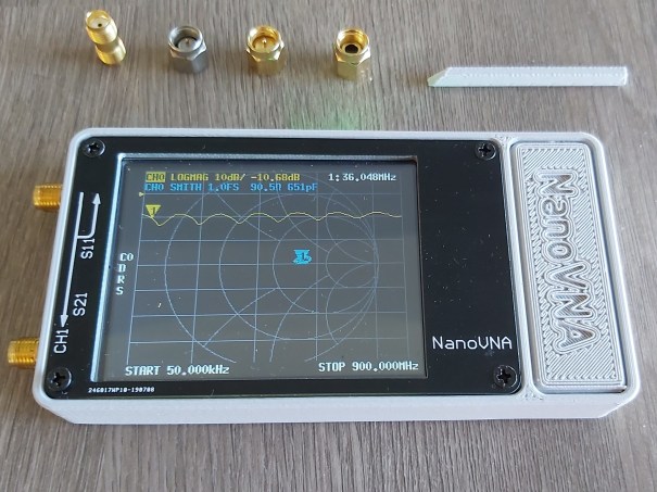
NanoVNA with cal standards. From L to R, Thru, Load(51Ω), Short, Open.

The NanoVNA has generated a fair amount of interest over the past couple of months and after a few days playing with it I can see why. Number 1, it’s cheap. I only paid about £50 for my model. Secondly, it actually works fairly well and has a reasonable frequency range. I have tried some other low cost VNAs in the past and been very disappointed.

Features

• S11 and S21 measurements. Sometimes called a 2 port, non-reversing VNA.
• 50KHz to 900MHz Range – (best accuracy upto 300MHz.)
• Touchscreen control
• Multiple plot views.
• PC control and export of Touchstone files. An industry standard VNA file format.

I made a nice case for my unit. You can find the model on thingyverse.

There are a few missing features, but you probably won’t need these and can work normally work around them.

Missing Features

• 101 sweep points only. No way to change this currently, so on a wideband sweep, you can easily miss narrowband features. There is now some beta software that specifically addresses this.
• No output power sweep. Useful for characterising non-linear devices.
• Slow sweep speed. About 10ms per point. The basic Copper Mountain VNA is about 100x faster. Believe me fast sweeps are a really helpful.
• Time Domain Reflectometry. You can do this in post-processing . Lots of professional high-end VNAs do not have this feature charge extra for this feature. Not sure why, it’s only a trivial IFFT. There is now some beta software that specifically addresses this.
• No de-embedding. 99.9% of people will never need this.
• Limited PC software.
• Limited frequency range. A lot of people will miss it not covering 915MHz and even more will miss 2.4GHz.
• The cal kit and cables that come with the kit are pretty cheap and nasty. That said, most pro VNAs don’t include cables or cal kits at all. These generally cost extra, and aren’t cheap.
• Calibration assumes ‘ideal’ calibration standards. Professional kits come with correction coefficients that allow more accurate calibration. Probably not a problem for most people working below 900MHz.

That’s really just nitpicking though. For the price, there is a lot of bang for buck here. For general radio HAM bands, this thing is great.

Setup and Calibration

Calibration is vital for all VNA’s, and especially so for older and low cost VNA’s like this. Modern expensive VNAs are actually remarkable good in the preset state and you can often get away with making simple scaler measurements with short cables without running through the calibration routine. For this I would highly recommend calibrating every time.

Step 1 – Set the frequency range.

The nanoVNA only has 101 sweep points, so to get accurate measurements, it best to set up your frequency sweep before calibrating.

Set the frequency range under the Stimulus menu.

Choose start, stop centre or span.

Top tip. Using the rocker control or the clicking on the displayed frequency is nearly impossible. The user interface doesn’t give much clue, but you can press on this blank region to bring up a keypad.

Press here to bring up the keypad.

Congratulations, You have unlocked the secret keypad!

The keypad makes it much easier to select your desired frequency. Use x1 for Hz, K for kilohertz, M for megahertz and not sure why you would need it, but gigahertz is there too.

Step 2 – Connect your cables/Define your reference plane.

Ideally we want to calibrate our VNA as close as possible to the device under test. Unless the cable is the device we wish to test that is.

If you wish to do S21 measurements, you will probably need to connect a cable to both ports. If you only need S11 measurements and are able to connect your device directly then you might be able to do without the cables.

Dependent upon what you are doing, it can be very important to understand where the reference plane[see below] of you VNA is. For instance, if we are designing an impedance matching network and are using our S11 measurement to work out what value of inductance of capacitance to add, by default this will only be valid if we place the component at the same location we calibrated for. Don’t be surprised if you add an inductor 3 inches from you cal point and find it doesn’t do what you expected. You can add a manual delay into the calibration to compensate for this(it’s hidden in the Scale menu). I won’t go into that for this blog though.

“Reference Plane” -Because signals travel through cables and circuits at a finite speed. The relative phase measurements will change the as you move away from the point of calibration. On the smith chart this results in the vector being rotated around the graph. By default the reference plane is the same as the calibration point, but we can use software tricks to extend the reference plane either towards of away from the VNA. At 900MHz(333mm wavelength) the ~5mm length of the connector represents ~5° of phase difference, so depending on your measurement needs you may need to work out exactly where inside your connector the calibration is valid.

Step 3 – Conduct the calibration.

Tip – Reset first. Especially if you just conduct an Open, Short Load cal, rather than the full Isolation and Thru measurements.

Short,Open-Load. Connect the Open to the end of the cable on your S11 port and press OPEN. Repeat this for each calibration standard. Note, the OPEN standard is not required and can actually be left unconnected. User tests have shown that this actually results in a more accurate calibration due to extra capacitance effects of the included Open connector.

Open, Short and Load Standards next to their associated calibration menu.

Isolation – Connect the Load to the S21(CH1) port and press ISOLN.

Thru – Connect the S11 cable to S21(CH1). Depending on your cables you may need to use the female to female slug that hopefully your kit came with. In expensive VNA’s this thru standard has calibration data so the VNA can remove the small level of attenuation and extra length this adaptor introduces. For the NanoVNA, we normally just have to accept the small error it introduces.

Step 4 – Final Check

Use each of your cal standards once more to make sure it worked.

Short: -Smith chart should all be grouped on the very left hand side of the chart on the centre line. LOGMAG plot should read close to 0dB.

Open: – Smith chart should all be grouped on the very right hand side of the chart on the centre line. LOGMAG plot should read close to 0dB.

Load: – Smith chart should be grouped around the centre of the plot. LOGMAG Plot should be showing a low number (-50dB or below)

In the next blog I hope to present some guidance on how to configure your channels for S11 or S21 as well showing some examples of using this VNA.